Information retrieval model
Download as pptx, pdf3 likes3,602 views

情報検索モデル 原著者とアップロード者は別人です。 原著者の許可を得た上でアップロードしています。


![[DL輪読会]Deep Reinforcement Learning that Matters](https://cdn.slidesharecdn.com/ss_thumbnails/deeprlthatmatters-171212050658-thumbnail.jpg?width=560&fit=bounds)


![[GTCJ2018]CuPy -NumPy互換GPUライブラリによるPythonでの高速計算- PFN奥田遼介](https://cdn.slidesharecdn.com/ss_thumbnails/gtcj2018cupypfnryosukeokuta-181009073034-thumbnail.jpg?width=560&fit=bounds)


![[DL輪読会]GLIDE: Guided Language to Image Diffusion for Generation and Editing](https://cdn.slidesharecdn.com/ss_thumbnails/glide2-220107030326-thumbnail.jpg?width=560&fit=bounds)


More Related Content
What's hot (20)
Viewers also liked (20)


![[data analytics showcase] B14: 文字情報の分析基盤 Mroonga by 株式会社インサイトテクノロジー 小幡 一郎](https://cdn.slidesharecdn.com/ss_thumbnails/gewtegxitccqr9e2hb5m-signature-dbdadd8978e07a8eac70e8d97843d87d84136d17cf5a5b684423cc574b8995e4-poli-161007060519-thumbnail.jpg?width=560&fit=bounds)
Similar to Information retrieval model (20)


Information retrieval model
- 1. 情報検索モデル勉強会 D2 加藤 誠
- 2. • 全てのコンテンツが有用とは限りません – 聞きたいときだけ聞いて聞かないときは聞か ないことをお勧めします – 自分の研究と照らし合わせてみてください • 知りたいけどわからない場合は遠慮なく 聞いてください – 完全インタラクティブ制です • スライドでは重要な情報が欠けている場合があり ます 2
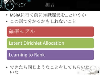
- 3. • MSRAに行く前に知識還元を…というか • この話で分かるかもしれないこと 確率モデル Latent Dirichlet Allocation Learning to Rank • できたら同じようなことをしてもらいた いな 3
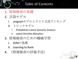
- 4. 1. 情報検索の基礎 2. 言語モデル I. unigramモデルとクエリ尤度ランキング II. トピックモデル i. Probabilistic Latent Semantic Analysis ii. Latent Dirichlet Allocation 3. 情報検索のための機械学習 I. SVMの基礎 II. Learning to Rank 4. (情報検索の評価手法) 4
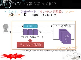
- 5. • クエリ,対象データ,ランキング関数,フレー Q ムワーク D Rank: Q x D -> R クエリ システム ランキングされたデータ 対象 デー タ ランキング関数 フレームワーク Baeza-Yates, R. and Ribeiro-Neto, B. and others, Modern Information Retrieval より 注: 狭義です 5
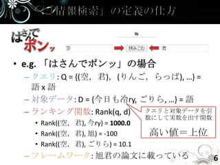
- 6. • e.g. 「はさんでポンッ」の場合 – クエリ: Q = {(空,君),(りんご,らっぱ), …} = 語x語 – 対象データ: D = {今日も冷ry, ごりら, …} = 語 – ランキング関数: Rank(q, d) クエリと対象データを引 数にして実数を出す関数 • Rank((空,君), 今ry) = 1000.0 • Rank((空,君), 旭) = -100 高い値=上位 • Rank((空,君), ごりら) = 10.1 – フレームワーク: 旭君の論文に載っている 6
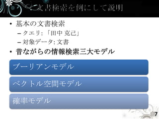
- 7. • 基本の文書検索 – クエリ: 「田中 克己」 – 対象データ: 文書 • 昔ながらの情報検索三大モデル ブーリアンモデル ベクトル空間モデル 確率モデル 7
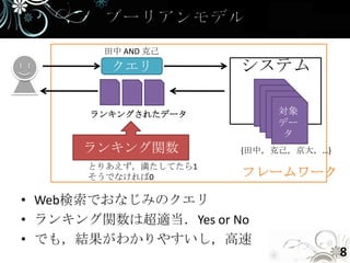
- 8. 田中 AND 克己 クエリ システム ランキングされたデータ 対象 デー タ ランキング関数 {田中,克己,京大,…} とりあえず,満たしてたら1 そうでなければ0 フレームワーク • Web検索でおなじみのクエリ • ランキング関数は超適当.Yes or No • でも,結果がわかりやすいし,高速 8
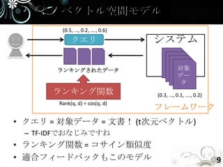
- 9. (0.5, …, 0.2, …., 0.6) クエリ システム ランキングされたデータ 対象 デー タ ランキング関数 (0.3, …, 0.1, …., 0.2) Rank(q, d) = cos(q, d) フレームワーク • クエリ = 対象データ = 文書! (t次元ベクトル) – TF-IDFでおなじみですね • ランキング関数 = コサイン類似度 • 適合フィードバックもこのモデル 9
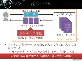
- 10. (1,0, 0, …, 1, …., 0, 1) クエリ システム ランキングされたデータ 対象 デー タ ランキング関数 (0,0, 1, …, 1, …., 1, 0) Rank(q, d) = P(R|d) / P(NR|d) フレームワーク • クエリ,対象データ: ある語wiが入ってたら1,入ってな かったら0 – e.g. w1 = 田中,w2 = 克己,w3 = 情報学,{田中,克己} = (1, 1, 0) • ランキング関数 = 文書dが適合文書である確率/不適合である確率 10
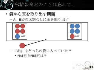
- 11. • 袋から玉を取り出す問題 – A,B袋の区別なしに玉を取り出す A袋 B袋 – 「赤」はどっちの袋に入っていた? • P(A|赤)とP(B|赤)は? 11
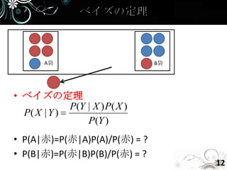
- 12. A袋 B袋 • ベイズの定理 P(Y | X ) P( X ) P( X | Y ) P(Y ) • P(A|赤)=P(赤|A)P(A)/P(赤) = ? • P(B|赤)=P(赤|B)P(B)/P(赤) = ? 12
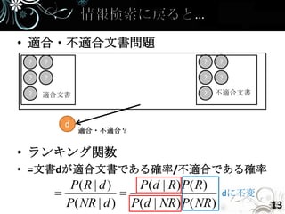
- 13. • 適合・不適合文書問題 ? ? ? ? ? ? ? ? ? 適合文書 ? 不適合文書 d 適合・不適合? • ランキング関数 • =文書dが適合文書である確率/不適合である確率 P( R | d ) P(d | R) P( R) dに不変 P( NR | d ) P(d | NR ) P( NR ) 13
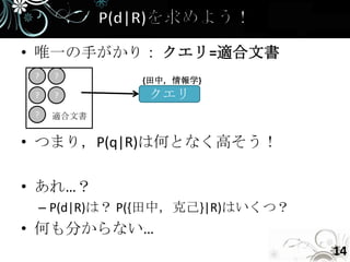
- 14. • 唯一の手がかり: クエリ=適合文書 ? ? {田中,情報学} ? ? クエリ ? 適合文書 • つまり,P(q|R)は何となく高そう! • あれ…? – P(d|R)は? P({田中,克己}|R)はいくつ? • 何も分からない… 14
- 15. • 何か仮定が必要です 15
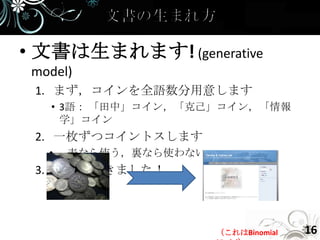
- 16. • 文書は生まれます! (generative model) 1. まず,コインを全語数分用意します • 3語: 「田中」コイン,「克己」コイン,「情報 学」コイン 2. 一枚ずつコイントスします • 表なら使う,裏なら使わない 3. 文書ができました! (これはBinomial 16
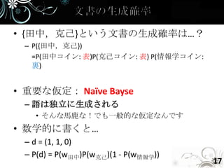
- 17. • {田中,克己}という文書の生成確率は…? – P({田中,克己}) =P(田中コイン: 表)P(克己コイン: 表) P(情報学コイン: 裏) • 重要な仮定: Naïve Bayse – 語は独立に生成される • そんな馬鹿な!でも一般的な仮定なんです • 数学的に書くと… – d = (1, 1, 0) – P(d) = P(w田中)P(w克己)(1 - P(w情報学)) 17
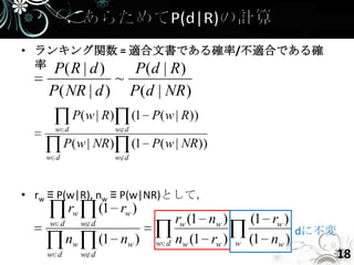
- 18. • ランキング関数 = 適合文書である確率/不適合である確 率 P( R | d ) P(d | R) ~ P( NR | d ) P(d | NR ) P( w | R) (1 P( w | R)) w d w d P( w | NR) (1 P( w | NR)) w d w d • rw ≡ P(w|R), nw ≡ P(w|NR)として, rw (1 rw ) w d w d rw (1 nw ) (1 rw ) dに不変 nw (1 nw ) w d nw (1 rw ) w (1 nw ) w d w d 18
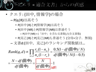
- 19. • クエリ: {田中, 情報学}の場合 – P(q|R)は高そう • P(田中|R)とP(情報学|R)は高そう • P(田中|NR)とP(情報学|NR)は普通そう – P(田中|NR) = (「田中」を含む文書数) / (全文書数) • P(克己|R)とP(克己|NR)も普通そう (分母=分子.無視) – 文書d:{田中,克己}のランキング関数値は… rw (1 nw ) 0.5(1 df (田中) / N ) Rank(q, d ) w d nw (1 rw ) df (田中) / N (1 0.5) N df (田中) N 1 df (田中) df (田中) idf! 19
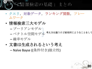
- 20. • クエリ,対象データ,ランキング関数,フレー ムワーク • 情報検索三大モデル – ブーリアンモデル 考え方は違うけど結局同じようなことをして – ベクトル空間モデル – 確率モデル • 文書は生成されるという考え – Naïve Bayse ((条件付き)独立性) 20
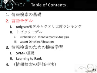
- 21. 1. 情報検索の基礎 2. 言語モデル I. unigramモデルとクエリ尤度ランキング II. トピックモデル i. Probabilistic Latent Semantic Analysis ii. Latent Dirichlet Allocation 3. 情報検索のための機械学習 I. SVMの基礎 II. Learning to Rank 4. (情報検索の評価手法) 21
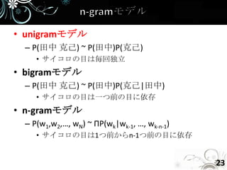
- 22. • 文書は生まれます! (今度はサイコ ロ) 1. まず,サイコロを用意します • 3語: 「田中」面,「克己」面,「情報学」面 2. 好きなだけ投げます • 出た目の語を使います 3. 文書ができました! さっきのコインも言語モデルだと思う(or 言語モデルによる説明) (これはMultinomial Model) 22
- 23. • unigramモデル – P(田中 克己) ~ P(田中)P(克己) • サイコロの目は毎回独立 • bigramモデル – P(田中 克己) ~ P(田中)P(克己|田中) • サイコロの目は一つ前の目に依存 • n-gramモデル – P(w1,w2,…, wN) ~ ΠP(wk|wk-1, …, wk-n-1) • サイコロの目は1つ前からn-1つ前の目に依存 23
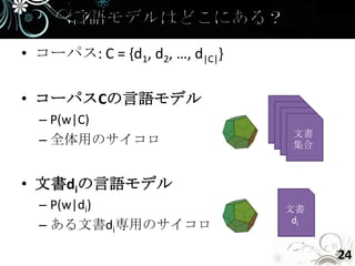
- 24. • コーパス: C = {d1, d2, …, d|C|} • コーパスCの言語モデル – P(w|C) 文書 – 全体用のサイコロ 集合 • 文書diの言語モデル – P(w|di) 文書 di – ある文書di専用のサイコロ 24
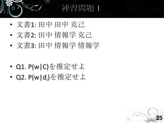
- 25. • 文書1: 田中 田中 克己 • 文書2: 田中 情報学 克己 • 文書3: 田中 情報学 情報学 • Q1. P(w|C)を推定せよ • Q2. P(w|di)を推定せよ 25
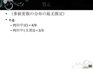
- 26. • (多値変数の分布の最尤推定) • e.g. – P(田中|C) = 4/9 – P(田中|文書1) = 2/3 26
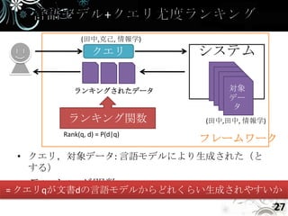
- 27. (田中,克己, 情報学) クエリ システム ランキングされたデータ 対象 デー タ ランキング関数 (田中,田中, 情報学) Rank(q, d) = P(d|q) フレームワーク • クエリ,対象データ: 言語モデルにより生成された(と する) • ランキング関数 = クエリqが文書dの言語モデルからどれくらい生成されやすいか 27
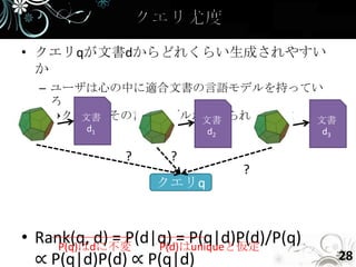
- 28. • クエリqが文書dからどれくらい生成されやすい か – ユーザは心の中に適合文書の言語モデルを持ってい る →クエリはその言語モデルから作られている! 文書 文書 文書 d1 d2 d3 ? ? ? クエリq • Rank(q, d) = P(d|q) = P(q|d)P(d)/P(q) P(q)はdに不変 P(d)はuniqueと仮定 ∝ P(q|d)P(d) ∝ P(q|d) 28
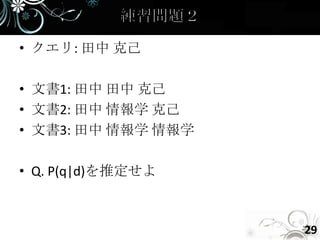
- 29. • クエリ: 田中 克己 • 文書1: 田中 田中 克己 • 文書2: 田中 情報学 克己 • 文書3: 田中 情報学 情報学 • Q. P(q|d)を推定せよ 29
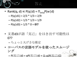
- 30. • Rank(q, d) ∝ P(q|d) = Πw∈qP(w|d) – P(q|d1) = 2/3 * 1/3 = 2/9 – P(q|d2) = 1/3 * 1/3 = 1/9 – P(q|d3) = 1/3 * 0 = 0!? • 文書d3が語「克己」をはき出す可能性は 0?? – ちょっと大げさな推定 • コーパスの言語モデルを使ったスムージ ング – P(克己|d) = αP(克己|d) + (1-α)P(克己|C) 30
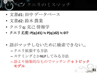
- 31. • 文書d1: 田中 データベース • 文書d2: 鈴木 農業 • クエリq: 克己 情報学 • クエリ尤度: P(q|d1) ≒ P(q|d2) ≒ 0!? • 語がマッチしないために検索できない… – クエリ拡張する方法 – ステミングとかNLPしてみる方法 – 語より抽象的なものでマッチング→ トピック モデル 31
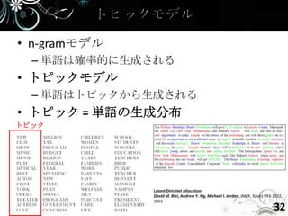
- 32. • n-gramモデル – 単語は確率的に生成される • トピックモデル – 単語はトピックから生成される • トピック = 単語の生成分布 トピック Latent Dirichlet Allocation David M. Blei, Andrew Y. Ng, Michael I. Jordan; JMLR, 3(Jan):993-1022, 2003. 32
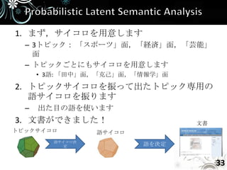
- 33. 1. まず,サイコロを用意します – 3トピック: 「スポーツ」面,「経済」面,「芸能」 面 – トピックごとにもサイコロを用意します • 3語: 「田中」面,「克己」面,「情報学」面 2. トピックサイコロを振って出たトピック専用の 語サイコロを振ります – 出た目の語を使います 3. 文書ができました! 文書 トピックサイコロ 語サイコロ 語サイコロ決 定 語を決定 33
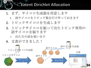
- 34. 1. まず,サイコロ生成器を用意します I. 語サイコロをトピック数分だけ作っておきます 2. トピックサイコロを生成します 3. トピックサイコロを振って出たトピック専用の 語サイコロを振ります – 出た目の語を使います 4. 文書ができました! 語サイコロ生成器 語サイコロ トピックサイコロ生成器 文書 トピックサイコロ 語サイコロ 語サイコロ決 定 語を決定 34
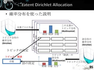
- 35. • 確率分布を使った説明 この文書の 文書ごとに生成 トピック分布 政治 経済 芸能 (Multinomial) 政治 経済 芸能 政治 経済 芸能 トピック分布の 語分布の 確率分布 確率分布 (Dirichlet) (Dirichlet) トピックの決定 トピック「経済」の トピック: 経済 語分布 市場 (Multinomial) トピックごとに生成 語の決定 野球 市場 大学 35
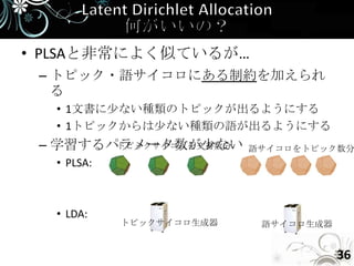
- 36. • PLSAと非常によく似ているが… – トピック・語サイコロにある制約を加えられ る • 1文書に少ない種類のトピックが出るようにする • 1トピックからは少ない種類の語が出るようにする – 学習するパラメータ数が少ない トピックサイコロを文書数分 語サイコロをトピック数分 • PLSA: • LDA: トピックサイコロ生成器 語サイコロ生成器 36
- 37. 注意:ここから難易度が上がりま す 37
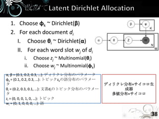
- 38. 1. Choose φk ~ Dirichlet(β) 2. For each document di I. Choose θi ~ Dirichlet(α) II. For each word slot wj of di i. Choose zj ~ Multinomial(θi) ii. Choose wj ~ Multinomial(φk) α, β = (0.1, 0.2, 0.3, …): ディリクレ分布のパラメータ φk = (0.1, 0.2, 0.3, …): トピックzkの語分布のパラメー タ ディリクレ分布=サイコロ生 θi = (0.2, 0.3, 0.1, …): 文書diのトピック分布のパラメー 成器 タ 多値分布=サイコロ zi = (0, 0, 0, 1, 0, …): トピック wi = (0, 1, 0, 0, 0, …): 語 38
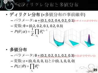
- 39. • ディリクレ分布 (=多値分布の事前確率) – パラメータ: α = (0.1, 0.2, 0.4, 0.2, 0.1) どのサイコロがでやすい – 変数: θ = (0.2, 0.2, 0.1, 0.2, 0.3) 1 – P( | ) k k 1 Z k • 多値分布 – パラメータ: θ = (0.2, 0.2, 0.1, 0.2, 0.3) どの目がでやすいか – 変数: z = (0, 0, 0, 0, 1)とか(0, 1, 0, 0, 0) zk – P( z | ) k zk 39
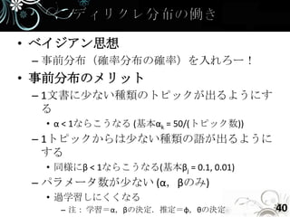
- 40. • ベイジアン思想 – 事前分布(確率分布の確率)を入れろー! • 事前分布のメリット – 1文書に少ない種類のトピックが出るようにす る • α < 1ならこうなる (基本αk = 50/(トピック数)) – 1トピックからは少ない種類の語が出るように する • 同様にβ < 1ならこうなる(基本βj = 0.1, 0.01) – パラメータ数が少ない (α,βのみ) • 過学習しにくくなる – 注: 学習=α,βの決定.推定=φ,θの決定 40
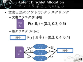
- 41. • 文書と語のソフト(共)クラスタリング – 文書クラスタ (P(z|θ)) 文書 d1 P(z|θ1) = (0.1, 0.3, 0.6) – 語クラスタ (P(z|w)) 田中 P(z|田中) = (0.2, 0.4, 0.4) トピッ 0.1 ク1 0.2 文書 0.3 トピッ 0.4 田中 d1 ク2 0.6 トピッ 0.4 ク3 41
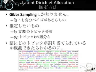
- 42. • Gibbs Samplingしか知りません… – 他にも変分ベイズがあるらしい • 推定したいもの – θi: 文書iのトピック分布 – φk: トピックkの語分布 • 語にどのトピックが割り当てられている か観測できたらわかるのに… 42
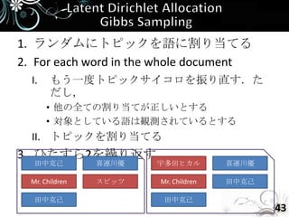
- 43. 1. ランダムにトピックを語に割り当てる 2. For each word in the whole document I. もう一度トピックサイコロを振り直す.た だし, • 他の全ての割り当てが正しいとする • 対象としている語は観測されているとする II. トピックを割り当てる 3. ひたすら2を繰り返す 田中克己 喜連川優 宇多田ヒカル 喜連川優 Mr. Children スピッツ Mr. Children 田中克己 田中克己 田中克己 43
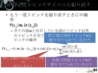
- 44. • もう一度トピックを振り直すときにの確 率 P(zi,j|w, (z-{zi,j})) – 全ての語wと注目している語のトピック以外 同じ語に何回トピックkが のトピックが全てわかっているときにそのト ピックの確率 割り当てられているか? n (v, k ) v P ( zi , j k | w, (z {zi , j })) (n(i, k ) k) ( n( r , k ) r ) r 同じ文書内で何回トピックk 全体で何回トピックkが が 出ているか? 割り当てられているか? 44
- 45. • 言語モデル – ユニグラムモデル – トピックモデル • Probabilistic Latent Semantic Analysis • Latent Dirichlet Allocation • クエリ尤度ランキング 45
- 46. 1. 情報検索の基礎 2. 言語モデル I. unigramモデルとクエリ尤度ランキング II. トピックモデル i. Probabilistic Latent Semantic Analysis ii. Latent Dirichlet Allocation 3. 情報検索のための機械学習 I. SVMの基礎 II. Learning to Rank 4. (情報検索の評価手法) 46
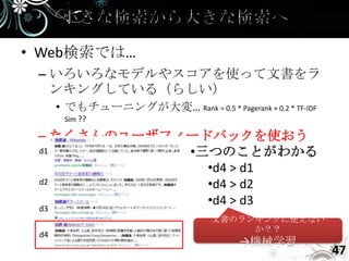
- 47. • Web検索では… – いろいろなモデルやスコアを使って文書をラ ンキングしている(らしい) • でもチューニングが大変… Rank = 0.5 * Pagerank + 0.2 * TF-IDF Sim ?? – たくさんのユーザフィードバックを使おう d1 •三つのことがわかる •d4 > d1 d2 •d4 > d2 •d4 > d3 d3 文書のランキングに使えない か?? d4 →機械学習 47
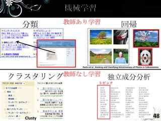
- 48. 分類 教師あり学習 回帰 78点 89点 ??点 21点 31点 ??点 Pedro et al., Ranking and Classifying Attractiveness of Photos in Folksonomies クラスタリング教師なし学習 独立成分分析 トピック Clusty 48
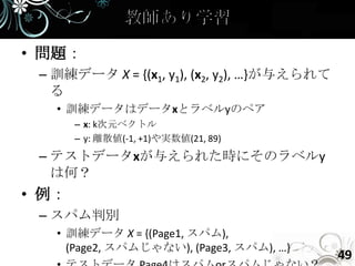
- 49. • 問題: – 訓練データ X = {(x1, y1), (x2, y2), …}が与えられて る • 訓練データはデータxとラベルyのペア – x: k次元ベクトル – y: 離散値(-1, +1)や実数値(21, 89) – テストデータxが与えられた時にそのラベルy は何? • 例: – スパム判別 • 訓練データ X = {(Page1, スパム), (Page2, スパムじゃない), (Page3, スパム), …} 49
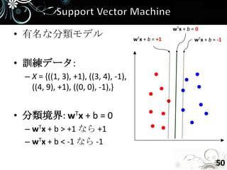
- 50. wTx + b = 0 • 有名な分類モデル wTx + b = +1 wTx + b = -1 • 訓練データ: – X = {((1, 3), +1), ((3, 4), -1), ((4, 9), +1), ((0, 0), -1),} • 分類境界: wTx + b = 0 – wTx + b > +1 なら +1 – wTx + b < -1 なら -1 50
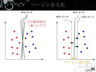
- 51. wTx + b = 0 wTx + b = 0 wTx + b = +1 wTx + b = -1 どの境界面が 一番いい?? マージン最大化 51
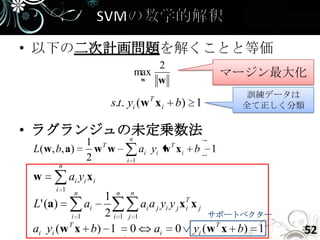
- 52. • 以下の二次計画問題を解くことと等価 2 max マージン最大化 w w T 訓練データは s.t. yi (w x i b) 1 全て正しく分類 • ラグランジュの未定乗数法 n 1 T L ( w , b, a ) w w ai yi w T x i b 1 2 i 1 n w ai y i x i i 1 n 1 n n L' (a) ai ai a j yi y j xT x j i i 1 2i 1 j 1 サポートベクター ai yi (w T x b) 1 0 ai 0 yi (w T x b) 1 52
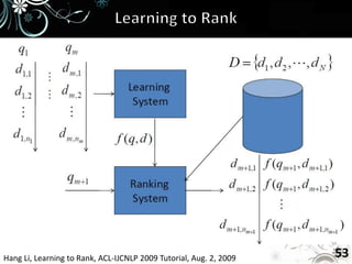
- 53. Hang Li, Learning to Rank, ACL-IJCNLP 2009 Tutorial, Aug. 2, 2009 53
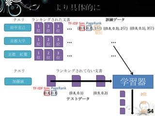
- 54. クエリ ランキングされた文書 訓練データ TF-IDF Sim. PageRank 田中克己 位 1 2 位 位 3 … ((0.9, 0.2), 1位) ((0.8, 0.3), 2位) ((0.8, 0.1), 3位) 順位 京都大学 1 位 2 位 3 位 … … 京都 紅葉 1 位 2 位 3 位 … … クエリ ランキングされてない文書 加藤誠 学習器 TF-IDF Sim. PageRank (0.8, 0.3) (0.8, 0.1) (0.9, 0.2) 2位 テストデータ 3位 1位 54
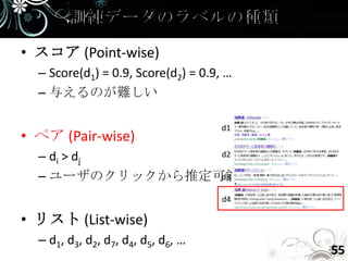
- 55. • スコア (Point-wise) – Score(d1) = 0.9, Score(d2) = 0.9, … – 与えるのが難しい d1 • ペア (Pair-wise) – di > dj d2 – ユーザのクリックから推定可能 d3 d4 • リスト (List-wise) – d1, d3, d2, d7, d4, d5, d6, … 55
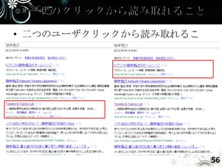
- 56. • 二つのユーザクリックから読み取れるこ とは? 56
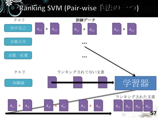
- 57. クエリ 訓練データ 田中克己 d1,1 > d1,2 d1,1 > d1,3 d1,3 > d1,2 京都大学 … 京都 紅葉 … クエリ ランキングされてない文書 加藤誠 学習器 ランキングされた文書 di,1 > di,2 di,3 > di,2 di,2 > di,4 di,1 di,3 di,4 di,2 57
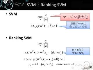
- 58. • SVM 2 max マージン最大化 w w T 訓練データは s.t. yi (w x i b) 1 全て正しく分類 • Ranking SVM 2 max w w T T di > djなら s.t. w xi w xj (di dj) wTxi > wTxj s.t. yi (wT (xi x j ) 0) 0 yi 1 (d i d j ) otherwise 1 58
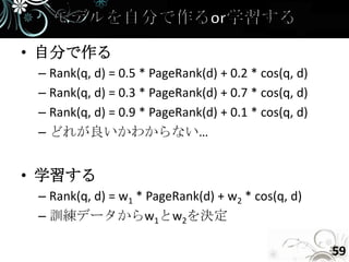
- 59. • 自分で作る – Rank(q, d) = 0.5 * PageRank(d) + 0.2 * cos(q, d) – Rank(q, d) = 0.3 * PageRank(d) + 0.7 * cos(q, d) – Rank(q, d) = 0.9 * PageRank(d) + 0.1 * cos(q, d) – どれが良いかわからない… • 学習する – Rank(q, d) = w1 * PageRank(d) + w2 * cos(q, d) – 訓練データからw1とw2を決定 59
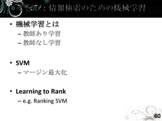
- 60. • 機械学習とは – 教師あり学習 – 教師なし学習 • SVM – マージン最大化 • Learning to Rank – e.g. Ranking SVM 60
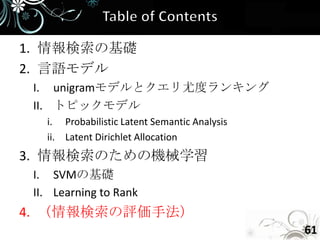
- 61. 1. 情報検索の基礎 2. 言語モデル I. unigramモデルとクエリ尤度ランキング II. トピックモデル i. Probabilistic Latent Semantic Analysis ii. Latent Dirichlet Allocation 3. 情報検索のための機械学習 I. SVMの基礎 II. Learning to Rank 4. (情報検索の評価手法) 61
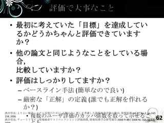
- 62. • 最初に考えていた「目標」を達成してい るかどうかちゃんと評価できています か? • 他の論文と同じようなことをしている場 合, 比較していますか? • 評価はしっかりしてますか? – ベースライン手法 (簡単なので良い) – 厳密な「正解」の定義 (誰でも正解を作れる か?) 酒井哲也: よりよい検索システム実現のために: 正解の良し悪しを考慮した情報検索評価の動向, 情報処理 Vol.47, No.2, pp.147- 158, 2006 • 複数のユーザ評価のカッパ係数を取って示せるこ 62 酒井哲也: チュートリアル:情報検索テストコレクションと評価指標, 情報処理学会研究報告 2008-FI-89 / 2008-NL-183, pp.1-8,
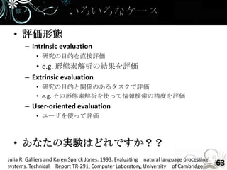
- 63. • 評価形態 – Intrinsic evaluation • 研究の目的を直接評価 • e.g. 形態素解析の結果を評価 – Extrinsic evaluation • 研究の目的と関係のあるタスクで評価 • e.g. その形態素解析を使って情報検索の精度を評価 – User-oriented evaluation • ユーザを使って評価 • あなたの実験はどれですか?? Julia R. Galliers and Karen Sparck Jones. 1993. Evaluating natural language processing systems. Technical Report TR-291, Computer Laboratory, University of Cambridge. 63
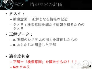
- 64. • タスク: – 検索意図: 正解となる情報の記述 – クエリ:検索意図を満たす情報を得るための クエリ • 正解データ: – A. 実際のシステムの出力を評価したもの – B. あらかじめ用意した正解 • 適合度判定 – 正解=「検索意図」を満たすもの!!! – Not クエリ 64
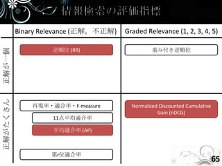
- 65. Binary Relevance (正解,不正解) Graded Relevance (1, 2, 3, 4, 5) 逆順位 (RR) 重み付き逆順位 正解が一個 正解がたくさん 再現率・適合率・F-measure Normalized Discounted Cumulative Gain (nDCG) 11点平均適合率 平均適合率 (AP) 第r位適合率 65
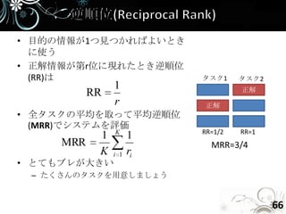
- 66. • 目的の情報が1つ見つかればよいとき に使う • 正解情報が第r位に現れたとき逆順位 (RR)は タスク1 タスク2 1 正解 RR r 正解 • 全タスクの平均を取って平均逆順位 (MRR)でシステムを評価 K RR=1/2 RR=1 1 1 MRR MRR=3/4 K i 1 ri • とてもブレが大きい – たくさんのタスクを用意しましょう 66
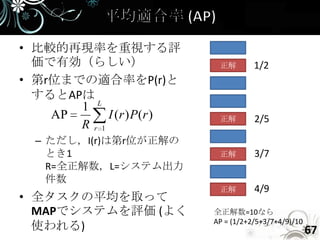
- 67. • 比較的再現率を重視する評 価で有効(らしい) 正解 1/2 • 第r位までの適合率をP(r)と するとAPは 1 L AP I (r ) P(r ) 正解 2/5 Rr1 – ただし,I(r)は第r位が正解の とき1 正解 3/7 R=全正解数,L=システム出力 件数 正解 4/9 • 全タスクの平均を取って MAPでシステムを評価 (よく 全正解数=10なら AP = (1/2+2/5+3/7+4/9)/10 使われる) 67
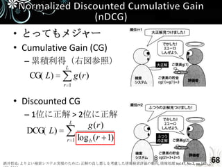
- 68. • とってもメジャー • Cumulative Gain (CG) – 累積利得(右図参照) L CG( L) g (r ) r 1 • Discounted CG – 1位に正解 > 2位に正解 L g (r ) DCG( L) r 1 log b ( r 1) 酒井哲也: よりよい検索システム実現のために: 正解の良し悪しを考慮した情報検索評価の動向, 情報処理 Vol.47, No.2, pp.147- 68
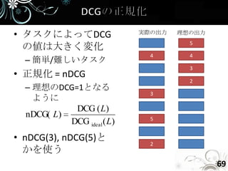
- 69. • タスクによってDCG 実際の出力 理想の出力 5 の値は大きく変化 4 4 – 簡単/難しいタスク 3 • 正規化 = nDCG 2 – 理想のDCG=1となる 3 ように DCG ( L) nDCG( L) 5 DCG ideal ( L) • nDCG(3), nDCG(5)と 2 かを使う 69
- 70. • α-nDCG – Diversityを考慮したnDCG – トピックごとにnDCGを出すらしい • 順位相関係数 – 適切な順位がわかっているときに利用 – ケンドールの順位相関係数 – スピアマンの順位相関係数 70
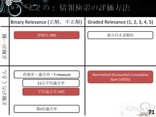
- 71. Binary Relevance (正解,不正解) Graded Relevance (1, 2, 3, 4, 5) 逆順位 (RR) 重み付き逆順位 正解が一個 正解がたくさん 再現率・適合率・F-measure Normalized Discounted Cumulative Gain (nDCG) 11点平均適合率 平均適合率 (AP) 第r位適合率 71
- 72. • 長々とすみません • Q&A? • 次の人はだれ? 72
- 73. • Modern Information Retrieval • Search Engines Information Retrieval in Practice • Introduction to Information Retrieval 73
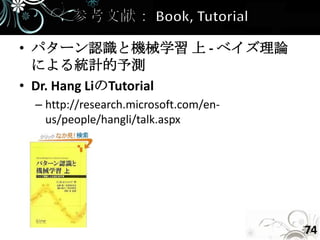
- 74. • パターン認識と機械学習 上 - ベイズ理論 による統計的予測 • Dr. Hang LiのTutorial – http://research.microsoft.com/en- us/people/hangli/talk.aspx 74
- 75. • Blei et al., Latent dirichlet allocation, JMLR • 酒井哲也氏の解説 – よりよい検索システム実現のために: 正解の 良し悪しを考慮した情報検索評価の動向 – 情報検索テストコレクションと評価指標 75