. 2014 Jul 24;511(7510):421-7.
doi: 10.1038/nature13595. Epub 2014 Jul 22.

Biological insights from 108 schizophrenia-associated genetic loci

Collaborators

Biological insights from 108 schizophrenia-associated genetic loci

Schizophrenia Working Group of the Psychiatric Genomics Consortium. Nature. .

Abstract

Schizophrenia is a highly heritable disorder. Genetic risk is conferred by a large number of alleles, including common alleles of small effect that might be detected by genome-wide association studies. Here we report a multi-stage schizophrenia genome-wide association study of up to 36,989 cases and 113,075 controls. We identify 128 independent associations spanning 108 conservatively defined loci that meet genome-wide significance, 83 of which have not been previously reported. Associations were enriched among genes expressed in brain, providing biological plausibility for the findings. Many findings have the potential to provide entirely new insights into aetiology, but associations at DRD2 and several genes involved in glutamatergic neurotransmission highlight molecules of known and potential therapeutic relevance to schizophrenia, and are consistent with leading pathophysiological hypotheses. Independent of genes expressed in brain, associations were enriched among genes expressed in tissues that have important roles in immunity, providing support for the speculated link between the immune system and schizophrenia.


Figures

Extended Data Figure 1
Extended Data Figure 1. Homogeneity of Effects Across Studies
Plot of the first two principal components (PC) from principal components analysis (PCA) of the logistic regression β coefficients for autosomal genome-wide significant associations. The input data were the β coefficients from 52 samples for 112 independent SNP associations (excluding 3 chrX SNPs and 13 SNPs with missing values in Asian samples). PCAs were weighted by the number of cases. Each circle shows the location of a study on PC1 and PC2. Circle size and colour are proportional to the number of cases in each sample (larger and redder circles correspond to more cases). Most samples cluster. Outliers had either small numbers of cases (“small”) or were genotyped on older arrays. Abbreviations. a500 (Affymetrix 500K); a5 (Affymetrix 5.0). Studies that did not use conventional research interviews are in the central cluster (CLOZUK, Sweden, and Denmark-Aarhus studies).
Extended Data Figure 2
Extended Data Figure 2. Quantile-quantile plot
Quantile-quantile plot of GWAS meta-analysis. Expected −log10(P) -values are those expected under the null hypothesis. For clarity, we avoided expansion of the Y-axis by setting association P-values < 10−12 to 10−12. The shaded area surrounded by a red line indicates the 95% confidence interval under the null. Lambda is the observed median χ2 test statistic divided by the median expected χ2 test statistic under the null.
Extended Data Figure 3
Extended Data Figure 3. LD Score regression consistent with polygenic inheritance
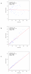
The relationship between marker χ2 association statistics and linkage disequilibrium (LD) as measured by the LD Score. LD Score is the sum of the r2 values between a variant and all other known variants within a 1 cM window, and quantifies the amount of genetic variation tagged by that variant. Variants were grouped into 50 equal-sized bins based on LD Score rank. LD Score Bin and Mean χ2 denotes mean LD score and test statistic for markers each bin. We simulated (Supplementary Text) test statistics under two scenarios: (a) no true association, inflation due to population stratification (b) polygenic inheritance (λGC =1.32), in which we assigned independent and identically distributed per-normalized-genotype effects to a randomly selected subset of variants. Panel (c) present results from the PGC schizophrenia GWAS (λGC =1.48). The real data are strikingly similar to the simulated data summarized in (b) but not (a). The intercept estimates the inflation in the mean χ2 that results from confounding biases, such as cryptic relatedness or population stratification. Thus, the intercept of 1.066 for the schizophrenia GWAS suggests that ~90% of the inflation in the mean χ2 results from polygenic signal. The results of the simulations are also consistent with theoretical expectation (see Supplementary Text).
Extended Data Figure 4
Extended Data Figure 4. Enrichment of Associations in Tissues and Cells
Genes whose transcriptional start is nearest to the most associated SNP at each schizophrenia-associated locus were tested for enriched expression in a) purified brain cell subsets obtained from mouse ribotagged lines. The red dotted line indicates P=0.05.
Extended Data Figure 5
Extended Data Figure 5. MGS Risk Profile Score Analysis
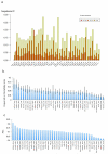
Polygenic risk profile score (RPS) analyses using the MGS sample as target, and deriving risk alleles from three published schizophrenia datasets (X-axis): ISC (2615 cases and 3338 controls) , PGC1 (excluding MGS, 9320 cases and 10,228 controls) , and the current meta analysis (excluding MGS) with 32,838 cases and 44,357 controls. Samples sizes differ slightly from original publication due to different analytical procedures. This shows the increasing RPS prediction with increasing training dataset size reflecting improved precision of estimates of the SNP effect sizes. The proportion of variance explained (Y-axis; Nagelkerke’s R2) was computed by comparison of a full model (covariates + RPS) score to a reduced model (covariates only). Ten different P-value thresholds (PT) for selecting risk alleles are denoted by the colour of each bar (legend above plot). For significance testing, see the bottom legend which denotes the P-value for the test that R2 is different from zero. All numerical data and methods used to generate these plots are available in Supplementary Tables 6, 7, and Supplementary Text.
Extended Data Figure 6
Extended Data Figure 6. Risk Profile Score Analysis
We defined 40 target subgroups of the primary GWAS dataset and performed 40 leave-one-out GWAS analyses (see Supplementary Material) from which we derived risk alleles for RPS analysis (X-axis) for each target subgroup. a) The proportion of variance explained (Y-axis; Nagelkerke’s R2) was computed for each target by comparison of a full model (covariates + RPS) score to a reduced model (covariates only). For clarity, 3 different P-value thresholds (PT) are presented denoted by the colour of each bar (legend above plot) as for Extended Data Figure 5 but for clarity we restrict to fewer P-value thresholds (PT of 5×10⁻⁸, 1×10⁻⁴, and 0.05) and removed the significance values. (b) The proportion of variance on the liability scale from risk scores calculated at the PT 0.05 with 95% CI bar assuming baseline population disease risk of 1%. (C) Area under the receiver operating curve (AUC). All numerical data and methods used to generate these plots are available in Supplementary Tables 6, 7, and Supplementary Text.
Extended Data Figure 7
Extended Data Figure 7. Epistasis
Quantile-quantile plot for all pair-wise (N=7750) combinations of the 125 independent autosomal genome-wide significant SNPs tested for non-additive effects on risk using case-control datasets of European ancestry (32,405 cases and 42,221 controls). We included as covariates the principal components from the main analysis as well as a study indicator. The interaction model is described by: Y=β0+β1X1+β2X2+β3X1X2+β4X4+β5X5 X1 and X2 are genotypes at the two loci, X1*X2 is the interaction between the two genotypes modeled in a multiplicative fashion, X4 is the vector of principal components, X5 is the vector of study indicator variables. Each β is the regression coefficient in the generalized linear model using logistic regression. The overall distribution of P-values did not deviate from the null and the smallest P-value (4.28×10⁻⁴) did not surpass the Bonferroni correction threshold (p=0.05/7750= 6.45×10⁻⁶). The line x=y indicates the expected null distribution with the grey area bounded by red lines indicating the expected 95% confidence interval for the null.
Figure 1
Figure 1. Manhattan plot
Manhattan plot of the discovery genome-wide association meta-analysis of 49 case control samples (34,241 cases and 45,604 controls) and 3 family based association studies (1,235 parent affected-offspring trios). The x-axis is chromosomal position and the y-axis is the significance of association (−log10(P)).The red line shows the genome-wide significance level (5×10⁻⁸). SNPs in green are in LD with the index SNPs (diamonds) which represent independent genome-wide significant associations.
Figure 2
Figure 2. Enrichment in enhancers
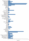
Cell and tissue type specific enhancers were identified using ChIP-seq datasets (H3K27ac signal) from 56 cell line and tissue samples (Y-axis). We defined cell and tissue type enhancers as the top 10% of enhancers with the highest ratio of reads in that cell or tissue type divided by the total number of reads. Enrichment of credible causal associated SNPs from the schizophrenia GWAS was compared with frequency matched sets of 1000 Genomes SNPs (Supplementary Text). The X-axis is the −log10(P) for enrichment. P-values are uncorrected for the number of tissues/cells tested. A −log10(P) of roughly 3 can be considered significant after Bonferroni correction. Descriptions of cell and tissue types at the Roadmap Epigenome website (http://www.roadmapepigenomics.org).
Figure 3
Figure 3. Odds ratio by risk score profile
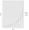
Odds ratio for schizophrenia by risk score profile (RPS) decile in the Sweden (Sw1-6), Denmark (Aarhus), and Molecular Genetics of Schizophrenia studies (Supplementary text). Risk alleles and weights were derived from ‘leave one out’ analyses in which those samples were excluded from the GWAS meta-analysis (Supplementary text). The threshold for selecting risk alleles was PT < 0.05. The RPS were converted to deciles (1=lowest, 10=highest RPS), and nine dummy variables created to contrast deciles 2-10 to decile 1 as the reference. Odds ratios and 95% confidence intervals (bars) were estimated using logistic regression with PCs to control for population stratification.

Comment in

Similar articles

  • Genetics: finding genes for schizophrenia.
    Flint J, Munafò MR. Flint J, et al. Curr Biol. 2014 Aug 18;24(16):R755-7. doi: 10.1016/j.cub.2014.07.018. Curr Biol. 2014. PMID: 25137590 Free PMC article.
  • Genome-wide analysis reveals extensive genetic overlap between schizophrenia, bipolar disorder, and intelligence.
    Smeland OB, Bahrami S, Frei O, Shadrin A, O'Connell K, Savage J, Watanabe K, Krull F, Bettella F, Steen NE, Ueland T, Posthuma D, Djurovic S, Dale AM, Andreassen OA. Smeland OB, et al. Mol Psychiatry. 2020 Apr;25(4):844-853. doi: 10.1038/s41380-018-0332-x. Epub 2019 Jan 4. Mol Psychiatry. 2020. PMID: 30610197 Free PMC article.
  • Genetic evidence for role of integration of fast and slow neurotransmission in schizophrenia.
    Devor A, Andreassen OA, Wang Y, Mäki-Marttunen T, Smeland OB, Fan CC, Schork AJ, Holland D, Thompson WK, Witoelar A, Chen CH, Desikan RS, McEvoy LK, Djurovic S, Greengard P, Svenningsson P, Einevoll GT, Dale AM. Devor A, et al. Mol Psychiatry. 2017 Jun;22(6):792-801. doi: 10.1038/mp.2017.33. Epub 2017 Mar 28. Mol Psychiatry. 2017. PMID: 28348379 Free PMC article. Review.
  • Common schizophrenia alleles are enriched in mutation-intolerant genes and in regions under strong background selection.
    Pardiñas AF, Holmans P, Pocklington AJ, Escott-Price V, Ripke S, Carrera N, Legge SE, Bishop S, Cameron D, Hamshere ML, Han J, Hubbard L, Lynham A, Mantripragada K, Rees E, MacCabe JH, McCarroll SA, Baune BT, Breen G, Byrne EM, Dannlowski U, Eley TC, Hayward C, Martin NG, McIntosh AM, Plomin R, Porteous DJ, Wray NR, Caballero A, Geschwind DH, Huckins LM, Ruderfer DM, Santiago E, Sklar P, Stahl EA, Won H, Agerbo E, Als TD, Andreassen OA, Bækvad-Hansen M, Mortensen PB, Pedersen CB, Børglum AD, Bybjerg-Grauholm J, Djurovic S, Durmishi N, Pedersen MG, Golimbet V, Grove J, Hougaard DM, Mattheisen M, Molden E, Mors O, Nordentoft M, Pejovic-Milovancevic M, Sigurdsson E, Silagadze T, Hansen CS, Stefansson K, Stefansson H, Steinberg S, Tosato S, Werge T; GERAD1 Consortium; CRESTAR Consortium; Collier DA, Rujescu D, Kirov G, Owen MJ, O'Donovan MC, Walters JTR. Pardiñas AF, et al. Nat Genet. 2018 Mar;50(3):381-389. doi: 10.1038/s41588-018-0059-2. Epub 2018 Feb 26. Nat Genet. 2018. PMID: 29483656 Free PMC article.
  • The polygenic architecture of schizophrenia - rethinking pathogenesis and nosology.
    Smeland OB, Frei O, Dale AM, Andreassen OA. Smeland OB, et al. Nat Rev Neurol. 2020 Jul;16(7):366-379. doi: 10.1038/s41582-020-0364-0. Epub 2020 Jun 11. Nat Rev Neurol. 2020. PMID: 32528109 Review.

Cited by

References

    1. Saha S, Chant D, McGrath J. A systematic review of mortality in schizophrenia: is the differential mortality gap worsening over time? Archives of General Psychiatry. 2007;64:1123–31. - PubMed
    1. World Health Organization . The Global Burden of Disease: 2004 Update. WHO Press; Geneva: 2008.
    1. Knapp M, Mangalore R, Simon J. The global costs of schizophrenia. Schizophrenia Bulletin. 2004;30:279–93. - PubMed
    1. Lieberman JA, et al. Effectiveness of antipsychotic drugs in patients with chronic schizophrenia. N Engl J Med. 2005;353:1209–23. - PubMed
    1. Carlsson A, Lindqvist M. Effect of Chlorpromazine or Haloperidol on Formation of 3methoxytyramine and Normetanephrine in Mouse Brain. Acta Pharmacologica et Toxicologica. 1963;20:140–4. - PubMed

Publication types