In my previous post, I asked about the following code and what its output will be:

As it turns out, this code will output two different numbers:

• On Debug – 134,284,904
• On Release – 66,896

The behavior is consistent between these two modes.

I was pretty sure that I knew what was going on, but I asked to verify. You can read the GitHub issue if you want the spoiler.

I attached to the running program in WinDBG and issued the following command:

We care about the last line. In particular, we can see that all the memory is indeed in the byte array, as expected.

Next, let’s dump the actual instances that take so much space:

There is one large instance here that we care about, let’s see what is holding on to this fellow, shall we?

It looks like we have a reference from a local variable. Let’s see if we can verify that, shall we? We will use the clrstack command and ask it to give us the parameters and local variables, like so:

The interesting line is 16, which shows:

In other words, here is the local variable, and it is set to null. What is going on? And why don’t we see the same behavior on release mode?

As mentioned in the issue, the problem is that the JIT introduce a temporary local variable here, which the GC is obviously aware of, but WinDBG is not. This cause the program to hold on to the value for a longer period of time than expected.

In general, this should only be a problem if you have a long running loop. In fact, we do in some case, and in debug mode, that actually caused our memory utilization to go through the roof and led to this investigation.

In release mode, these temporary variables are rarer (but can still happen, it seems).

Consider the following code:

Can you tell me what the output will be? And why?

On Oct 18, Rodrigo is going to talk about how a quick service restaurant chain has moved 36,000 locations (and millions of instances) from RavenDB 2.5 to 4.1.

In this session you will learn:

• Why RDI Software chose RavenDB for its quick service restaurant platform?
• All the hurdles that massive-scale deployments add to the mix
• How the migration to Version 4.0 enables the future vision of our platform?
• What were the trade-offs we had to make in moving from one version to the next?

Please register for the webinar in advance.

The fallacies of distributed computing is a topic that is very near and dear to my heart. These are a set of assertions describing false assumptions that distributed applications invariably make.

The first two are:

• The network is reliable.
• Latency is zero.

Whenever I talk about distributed computing, the fallacies come up. And they trip people up, over and over and over again. Even people who should know better.

Which is why I read this post with horror. That was mostly for the following quote:

As networks become more redundant, partitions become an increasingly rare event. And even if there is a partition, it is still possible for the majority partition to be available. Only the minority partition must become unavailable. Therefore, for the reduction in availability to be perceived, there must be both a network partition, and also clients that are able to communicate with the nodes in the minority partition (and not the majority partition).

Now, to be clear, Daniel literally has a PHD in CS and has published several papers on the topic. It is possible that he is speaking in very precise terms that don’t necessary match to the way I read this statement. But even so, I believe that this statement is absolutely and horribly wrong.

A network partition is rare, you say? This reading from 2014 paper for ACM Queue shows that this is anything but. Oh, sure, in the grand scheme of things, a network partition is an extremely rare event in a properly maintained data center, let’s say that this is a 1 / 500,000 chance for that happening (rough numbers from the Google Chubby paper). That still gives you 61 outages(!) in a few weeks.

Go and read the ACM paper, it makes for fascinating reading, in the same way you can’t look away from a horror movie however much you want to.

And this is talking just about network partitions. The problem is that from the perspective of the individual nodes, that is not nearly the only reason why you might get a partition:

• If running a server using a managed platform, you might hit a stop the world GC collection event. In some cases, this can be minutes.
• In an unmanaged language, your malloc() may be doing maintenance tasks and causing an unexpected block in a bad location.
• You may be swapping to disk.
• The OS might have decided to randomly kill your process (Linux OOM killer).
• Your workload has hit some critical point (see the Expires section) and cause the server to wait a long time before it can reply.
• Your server is on a VM that was moved between physical machines.
• A certificate expired on one machine, but not on others, meaning that it can contact others, but cannot be contacted directly (except that already existing connections still work).

All of these are before we consider the fact that we are dealing with imperfect software and that there may be bugs, that humans are tinkering with the system (such as deploying a new version) and mess things up, etc.

So no, I utterly reject the idea that partitions are rare events in any meaningful manner. Sure, they are rare, but a million to one event? We can do million packets per second. That means that something that is incredibly rare can still happen multiple times a day. In practice, you need to be aware that your software will be running in a partition, and that you will need a way to handle that.

And go read the fallacies again, maybe print them and stick them on a wall somewhere near by. If you are working with a distributed system, it is important to remember these fallacies, because they will trip you up.

One of the most important design decisions we made with RavenDB is not forcing users to explicitly create edges between documents. Instead, the edges are actually just normal properties on the documents and can be used as-is. This means that pretty much any existing RavenDB database can immediately start using graph operations, you don’t need to do anything.

The image below shows an order, using the RavenDB’s sample Northwind dataset. The highlighted portions mark the edges from this document. You can use these to traverse the graph by hopping from document to document.

For example, using:

This is easy to do, migrates well (zero cost to do so, yeah!) and usually matches nicely with what you already have. It does lead to an interesting observation. Typically, in a graph DB, you’ll model everything as a graph. But with RavenDB, you don’t need to do that.

In particular, let’s take a look at the Neo4J’s rendition of Northwind:

As you can see, everything is modeled as a node / edge. This is the only thing you could model it as. With RavenDB, you would typically use a domain driven model. In this case, it means that a value object, like an OrderLIne, will not have its own concrete existence. Either as a node or an edge. Instead, it will be embedded inside its root aggregate (the order).

Note that this is actually quite interesting, because it means that we need to be able to provide the ability to query on complex edges, such as the order lines. Here is how works:

This will give us all the discount products sold in London as well as their discount rate.

Note that in here, unlike previous queries, we use an named alias for the edge. In this case, it gives us the ability to access it properties and project the line’s Discount property to the user. This means that you can have a domain model with strong cohesion and locality, following the domain driven design principles while still being able to run arbitrary graph queries on it.  Combining this with the ability to pull data from indexes (including map/reduce) ones, you have a lot of things that you can do that used to be very hard but now are easy.

A query has two audiences: the users and the query engine. Ideally, you need to come up with a query language that would serve both. One of the early decisions that we made with the query language is that we want to be:

• Very flexible for the user, giving them several ways to express themselves.
• Be very rigid in the query engine, with only one way to do something.

These two requirements are directly contradicting one another, which is indeed somewhat of a problem. The key here is that we don’t want to produce multiple ways to do the same thing in the query engine. That is a great way to introduce:

• Different actual execution plans.
• Features that only work with a specific syntax.
• More complexity overall.

Anyone who ever worked with the internals of Linq can attest to the complexity that is involved here.

Let’s take the simple query that we have been inspecting so far:

Now, let’s ask RavenDB to spit it back out for us, shall we? Here is how RavenDB thinks about this query:

In other words, the way RavenDB sees the query and the way the user sees the query are very different. You can see that we have the with edges clauses here, defining the edges on the query.

In other words, all of the query definitions are happening in the with and with edges clauses. When we need to actually perform the matches, the match clause only defines the graph pattern that we need to match on.  It is the responsibility of the query parser to arrange the query from the multiple ways that the user may want to define it to the single representation that is actually going to be executed by the query runner.

This may seem like a lot of ceremony, but that is only because we have a very simple query. Let’s change the “friends of friends who aren’t my friends” to something a bit more interesting: “Close friends of my close friends who aren’t my friends”. We are also going to want to limit the friends that we follow only to Users (so, for example, we’ll not follow a FriendOf link to a Pet).

Here is what the query looks like, when we use more concise syntax, and how RavenDB translates it:

You’ll note that even for the query above, I still used a separate with clause to make things easier, the following query is exactly the same:

The basic idea is that for trivial filtering, you’ll probably want to do that inline, inside the match clause. But anything more complex should go to the with clause where you can more easily express your logic.  Also note that aliases matter. The f1 and f2 here are not duplicated for no reason, part of processing the query is to bind a value to each of the aliases, and you cannot bind a single result to multiple aliases.

Another key aspect of this mode is that while this is pretty easy to follow, a with clause can contain any query. That means that you can use indexes as well, including Map/Reduce indexes. Here is one such example:

In this case, I”m not sure how good a graph query this is, I’ll admit, but it does a good job of demonstrating what you can do. We are taking a few queries, mixing them together and then mashing the results to find London companies who didn’t order as much as they used to.

This means that the source information for graph queries can be things like spatial queries, full text search, map/reduce, etc. A lot of the complexity in graphs queries is just getting to do the start of the graph pattern matching. With RavenDB, you have a very strong query language and facilities to help you get past that and directly into the graph operations.

This is enough about the pre-processing the query, in my next post, I’m going to go into depth into how graph queries work with document models.

Pretty much all our early discussions about graphs in RavenDB focused on how to build the actual graph implementation. How to allow fast traversal, etc. When we started looking at the actual implementation, we realized that we seriously neglected a very important piece of the puzzle, the query interface for the graphs.

This is important for several reasons. First, ergonomics matter, if we end up with a query language that is awkward, it won’t see much use and complicate the users’ lives (and our own). Second, the query language effectively dictate how the user think about the model, so making low level decisions that would have impact on how the user is actually using this feature is probably not a good idea yet. We need to start from the top, what do we give to the user, and then see how we can make that a reality.

The most common use case of graph queries is the friends of friends query. Let’s see how this query is handled in various existing implementation, shall we?

Neo4J, using Cypher:

OrientDB doesn’t seem to have an easy way to do this. The following shows how you can find the 2nd degree friends, but it doesn’t exclude friends of friends who are already your friends. StackOverflow questions on that show scary amount of code, so I’m going to skip them.

Gremlin, which is used in a wide variety of databases:

We looked at other options, but it seems that graph query languages fall into the following broad categories:

• ASCII art to express the relationship between the nodes.
• SQL extensions that express the relationships as nested queries.
• Method calls to express the traversal.

Of the three options, we found the first option, using ASCII Art / Cypher as the easier one to work with. This is true both in terms of writing the query and actually executing it.

Let’s look at how friends of friends query will look like in RavenDB:

Graph queries are composed of two portions:

• With clauses, which determine source point for the graph traversal.
• Match clause (singular) that contain the graph pattern that we need to match on.

In the case, above, we are starting the graph traversal from start, this is defined as a with clause. A query can have multiple with clauses, each defining an alias that can be used in the match clause. The match clause, on the other hand, uses these aliases to decide how to process the query.

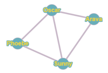
You can see that we have two clauses in the above query, and the actual processing is done by pattern matching (to me, it make sense to compare it to regular expressions or Prolog). It would probably be easier to show this with an example. Here is the relationship graphs among a few people:

We’ll set the starting point of the graph as Arava and see how this will be processed in the query.

For the first clause, we’ll have:

• start (Arava) –> f1 (Oscar) –> f2 (Phoebe)
• start (Arava) –> f1 (Oscar) –> f2 (Sunny)
• start (Arava) –> f1 (Sunny) –> f2 (Phoebe)
• start (Arava) –> f1 (Sunny) –> f2 (Oscar)

For the second clause, of the other hand, have:

• start (Arava) –> f2 (Oscar)
• start (Arava) –> f2 (Sunny)

These clauses are joined using and not operator. What this means is that we need to exclude from the first clause anything that matches on the second cluase. Match, in this case, means the same alias and value for any existing alias.

Here is what we need up with:

• start (Arava) –> f1 (Oscar) –> f2 (Phoebe)
• start (Arava) –> f1 (Oscar) –> f2 (Sunny) 
• start (Arava) –> f1 (Sunny) –> f2 (Phoebe)
• start (Arava) –> f1 (Sunny) –> f2 (Oscar)

We removed two entries, because they matched the entries from the second clause. The end result being just friends of my friends who aren’t my friends.

The idea with behind the query language is that we want to be high level and allow you to express what you want, and we’ll be in charge of actually making this work properly.

In the next post, I’ll talk a bit more about the query language, what scenarios it enables and how we are going to go about processing queries.

Note: These series of posts are about a planned feature, exploring how we go about building it. This is meant to solicit feedback and get more eyes on the idea, things aren’t set in stone and we don’t have a firm release date on this.

We have been wanting to add graph queries to RavenDB for several years now, but we always had more important things get in the way. That didn’t prevent us from discussing this internally and sketch up a few options. We are now looking at this more seriously and I thought that sharing the details of our deliberations would be interesting and likely to garner us some valuable feedback. I’m going to assume that the reader is at least somewhat familiar with the notion of graph data and graph queries.

Probably the most well known graph database is Neo4J, which provides the notion of nodes and edges, both of which have a type and a set of (flat) properties. This allow you to define a model of any arbitrary complexity. This works if you model is purely graph based, but it doesn’t work for RavenDB, whose users are used to the document model. On the surface, this looks like a minor detail. RavenDB has documents, which can have any shape, including containing embedded values and collections inside them. Neo4J, on the other hand, model things differently. The simplest example that I can think of is Orders and Order Lines, where you’ll have the following models:

Neo4J	RavenDB

Both models have the same information, but each element in the Neo4J graph is an independent node that is linked to the others. On the other hand, with RavenDB, we have a single document that embeds a lot of the information directly.  Note that what we haven’t shown in the image is that in RavenDB as well, you have other documents as well. The products, for example, are separate documents. 

Graph databases are often used to handle the basis of recommendation engines, fraud detection, etc. But they are usually used to augment the capabilities of the system, rather than as the primary data store of applications. RavenDB, on the other hand, is most frequently deployed as the primary data store. We want to give our users the ability to perform graph operations, but we don’t want to lose anything that make RavenDB useful and easy to use.

We initially thought about having the following definition:

• Each document is (implicitly) a node in the graph.
• You can call Link(src,dest,type, attributes) to create an edge between any two documents.
• Provide the usual graph queries on top of that.

We started exploring this implementation, but it quickly led to mounting complexity. From the point of view of the user, it led to having to do additional work, you’ll have to maintain your document model and the edges at the same time. This allow you to do some interesting things, but it also likely to cause complications down the line and very likely to cause issues when the document model and graph model disagree with one another. Other issues relates to how do you handle graphs in a distributed manner. How do you deal with the creation on an edge between two documents on one node when one of them was deleted on another?

We pushed in that direction for a while, because that was the obvious thing to do, but it really turned up to be a bad idea which didn’t play well with the rest of RavenDB. The worst part was the fact that you might modify the document properties but not define the edge, which lead to inconsistency. This was very easy to do.

The next thing we played with was to remove the Link() call and allow the user to define a background operation that would go and create the links between documents automatically whenever they were updated. This would allow us to avoid having any inconsistencies between the data in the documents and the links between then. After thinking about this for a while, we went ahead with this approach, but removed the requirement for a background operations.

RavenDB will be able to use your existing document model as the graph model as well. In other words, in the model above, you have the orders/2 document, which has two links, for each of the products. This give us both the ability to have a well define document model, with its well known Domain Driven architecture and the ability to hop off all the pre-existing links that we have in the model.

I’ll discuss the querying model and how it all plays together in a future post. For now, I want to show you how this looks like when we want to do a typical graph operation, friends of friends:

More details will come in the next post…

I run into this twit:

With the rise of asynchronous programming, debugging is getting much much harder. I met a couple of teams at Microsoft that explicitly avoid async because dump debugging is too hard.

— David Fowler (@davidfowl) August 26, 2018

This resonated very strongly with me, because when we architected RavenDB 4.0, one of the key considerations was the issue of debuggability. RavenDB instances often run for months on end, usually only restarted to apply updates to OS or database. They are often running in production environments where it is not possible to do any meaningful debugging. We rely heavily on resolving issues through minidumps, core dumps, etc. Part of the work we did in architecting RavenDB 4.0 was to sit down and think about supporting the system in production.

For many of the core components, async was right out. Part of that was because of issues relating to the unpredictability of async execution, we want certain things to always happen first, avoid thread pool starvation / growth policies / etc. But primarily, we were sick and tired of getting a dump (or even just pausing a running instance when we debug a complex situation) and having to manually reconstruct the state of the system. Parallel stacks alone is an amazing feature for figuring out what is going on in a complex system.

The design of RavenDB called for any long lived task to run on a dedicated thread. These threads are named, so if you stop in the debugger, you can very quickly see what is actually is going on there. This is also useful for things like account for memory, CPU time, etc. We had a problem in a particular component that was leaking memory at a rate of 144 bytes per second, just under 12 MB per day. This is something that is very easy to lose in the noise. But because we do memory accounting on a thread basis, it was easy to go to a system that was running for a few weeks and see that this particular thing had 500MB of memory in use, when we expected maybe 15MB.

We still use async for handling of short term operations. For example, processing of a single request, because these are fast and if there are problems with them, we’ll usually see them already executing.

I’m really happy with this decision, since it provided us many dividends down the line. We planned this for production, to be honest, but it ended up really helpful in normal debugging as well.

This also allow us to take advantage of the fact that a thread that is not runnable is effectively free (aside from some memory, of course), so we can dedicate a full thread for these long running tasks and greatly simplify everything. An index in RavenDB always has its own dedicated thread, which is woken up if there is anything that this index needs to process. This means that indexing code is simple, isolated and we can start applying policies at the index level easily. For example, if I have an index that has a low priority, I can just adjust the thread’s priority and let the OS do the hard work of scheduling it accordingly.

Async simplifies the programming model significantly, but it also come at a cost of system complexity and maintenance overhead. Figuring out that you have a request stuck on a task that will never return, for example, is never pleasant. The same thing using blocking operations is immediately obvious. That is a benefit that should absolutely not be discounted.

In my previous post, I talked about a task we give candidates that interview for the web developer position. They need to implement the following:

Given that I don’t like handing our tasks that I haven’t done, I took a few minutes to answer my own question. Here is how this can be implemented:

I believe that I mentioned that my JavaScript skills are from the last decade, if that, so I’m probably committing quite a few sins against JavaScript (if that is even possible), but this code run the first time I tried it and gave the proper result.